By Kilian Regan, Chief Product Officer, and Kevin Moses, Director of Operations, LDARtools
The year was 1996 and 11-year-old me (Kevin Moses), and my 9-year-old brother, were up to no good, or so we thought. Mom and Dad left us in the hands of our very capable teenage sister, who was undoubtedly talking on the cordless phone in her room. Recently Dad left a video in the VCR called “Fugitive Emissions” and this was the moment we had been waiting for.
Popcorn made, we sit down to what must certainly be a sequel to the 1993 Movie, “The Fugitive” with Harrison Ford. To our dismay, Harrison Ford never came on screen.
I presume an important part of the aforementioned video (which as one can guess, we did not finish), was the dark art of emissions reporting. Much later in life, I, along with Kilian Regan (co-author) had the opportunity to learn a great deal about emissions estimating from the great Graham “Buzz” Harris while working on the development of the
Chateau LDAR Software. There has been a lot of conversation recently about API fugitive emissions testing, but not as much about what happens after that. This article aims to share a high-level overview of how facilities report fugitive emissions to regulators.
Different Methods Available
The EPA provides a few ways emissions can be reported, and a facility must use the one that utilizes the best available data. Generally speaking, this will result in lower emissions being reported; the less data available, the more over-estimating will occur.
- The Correlation Equation method converts ppm to mass flow using equations provided by the EPA. This is the most common method used.
- The Average Emission Factors(AEF) method uses an industry average (generally determined by the EPA) to report unmeasured components. This method is used if components do not have monitoring (ppm) data.
- Others, such as >10,000ppm or < 10,000pmm (aka Leak, No Leak) OR AEF, are created using a facility’s historical data. These are largely unused and highly complex. They are mentioned only to highlight that they will not be covered in this overview.
The Correlation Equation
This method uses ppm values measured at each component in a correlation equation to report instantaneous emissions, then considers time in service (as well as some other factors) to get mass/time. The EPA has published the data needed to perform these calculations. Equations and values change based on industry, component type, and service.
- Zero Readings Emission Rates. Assumes there is a very small leak on 0 reading components.
- Peg Factors Emission Rates for analyzers that peg at 10,000ppm and 100,000ppm.
- The ppm Correlation Equation for everything in between 0 and analyzer peg.
The following is an example of a Valve in a refinery in Light Liquid Service:
- Zero Reading Emission Rate: 7.8E-6 kg/hr
- Pegged 10,000ppm: 0.064 kg/hr
- Pegged 100,000ppm: 0.14 kg/hr
- Correlation Equation: 2.29E-6(ppm)^0.746
Direct Measurement can also be used to replace or update the estimates. An example would be after finding a leak (ppm), another trip would be made to the component with a specialized device, such as a bagging kit or High Flow Sampler, that can capture all of the leak with a known amount of dilution. While the reading from the device is measured in concentration, the known dilution allows an accurate mass flow rate of the leak to be calculated.
Calculating Emissions Between Data Points
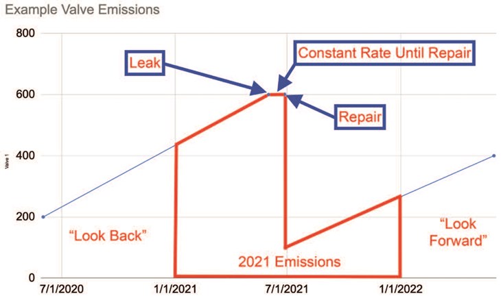
Linear interpolation (trapezoid) is the most commonly used calculation method and assumes that emission rates increase/decrease linearly between routine data points. As with almost everything about emission reporting of fugitives, the only thing known, is the likelihood it is not actually true. The change in the leak was almost certainly caused by an event, but there is no way to prove this with the data available.
There are exceptions to the linear assumption. One example is the emissions after a leak and before a repair attempt. The emissions rate is assumed to continue at the same rate until the repair attempt, as logic would suggest. See Chart 1 for an illustration of this.
Other methods of calculating the emissions between data points exist, but result in total emissions being essentially the same over time. The important issue is to not change calculation methods from one period to the next, as doing so could impact overall reported emissions.
One interesting thing about these calculations, as well as an example of complexity, is that data before and after the reporting period is needed to calculate the time-weighted emissions. For example, if a connector was monitored once in 2021, the calculator must look to 2020 data to get a starting point for the line. It will also look to 2022, and if there is no data yet, the line will continue straight. This means the calculated emissions for 2021 would change every time there is new monitoring on any annual component in 2022. See Chart 1 for an illustration of this.
Average Emission Factors
This is the simplest and most emissions overestimating method. It involves looking up a rate by industry, component type, and service, and multiplying by hours in service. It is used most commonly on connectors that do not require inspections or for heavy liquid components. There is almost always a large overreporting using this method as the emission factors were developed before any LDAR programs were in place, and used data from components that had never been inspected for leaks. In some cases, credits can be applied to this population of components if certain controls are in place.
Author’s Note
There are a lot of “always — except if” in the emissions estimating world. There is competing data published by the EPA, and the State Agencies, making it very complex. This article is a general overview of the art and is not intended to be advice or instruction. To learn more about fugitive emissions and how to handle this complexity, please contact an LDAR managing company.